The Bloom Filter is a probabilistic data structure designed to determine whether an item is or is not a member of a set. Its probabilistic nature grants it the ability to assert with certainty that an item is not part of the set, though it carries a probability of erroneously indicating that an item is in the set when it is not.
This phenomenon is known as a false positive, an inherent peculiarity to the Bloom Filter’s design, where collisions in data storage can lead to these inaccuracies. However, the Bloom Filter eliminates the possibility of false negatives, ensuring that if an item is not present, the structure will not return a false negative.
As more elements are added to the structure, the probability of having a false positive increases. However, this structure offers the flexibility to customize its parameters, allowing users to adjust and optimize the probability of collisions according to their needs.
Hash functions
Before explaining how it works, it’s important to briefly define what hash functions are, as they are key to understanding how the Bloom Filter functions.
Hash functions convert an input element into a distinct output element. The input is potentially infinite. On the other hand, the output is finite, meaning it is defined by a set of static bits. Another important feature is that if we apply the function to an input element, it will always produce the same output, meaning it is a pure function.
An infinite input and a finite output inevitably lead to collisions. Therefore, a good hash function must produce as few collisions as possible. How can this be measured? By the uniformity of the collisions. That is, the number of collisions per output should be homogeneous given a set of input data.
Although there are some bidirectional hash functions, the most useful and used are unidirectional. What does unidirectionality mean? That given an input, an output can be generated but given an output, the input cannot be retrieved. If we consider that there are an infinite number of inputs but a finite number of outputs, it means there are an infinite number of inputs for each possible output. Therefore, it is impossible to know the input value. Thanks to this property, hash functions are used to encrypt user passwords before storing them in databases.
Among the most used hash functions are SHA-256 and MD5. Each hash function provides a probability of collision as well as a computational cost. In general, the most used hash functions differ by computational cost and collision probability, allowing for the selection of the most appropriate one in each use case.
How does the bloom filter work?
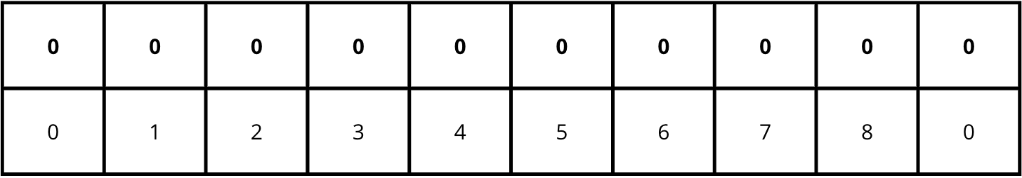
A Bloom Filter is defined by an m bit array (initially set to 0) and k different hash functions. These hash functions should be completely independent and have a low correlation.
When an item is added to the array, the k hash functions are applied. The result of each function indicates a position that must be marked with a 1 in the array.
In the case of a query, the process is similar; the k hash functions are applied to the input, and the values of the bits stored at those positions are retrieved. If one or more values are 0, then we can affirm that the item is NOT in the structure. If all values are 1s, then we can say that the item MIGHT be in the structure.
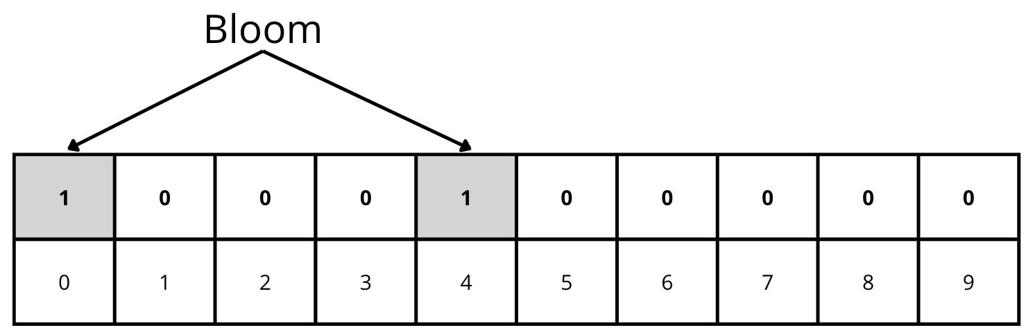
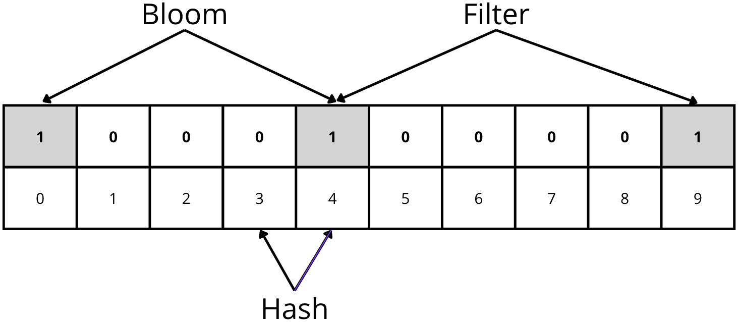
Starting with the 10-bit array in the previous image, let’s give some examples with two hash functions.
We add the word “Bloom” to the data structure, and applying the two hash functions gives us positions 0 and 4. In this case, we must mark both positions with a 1:
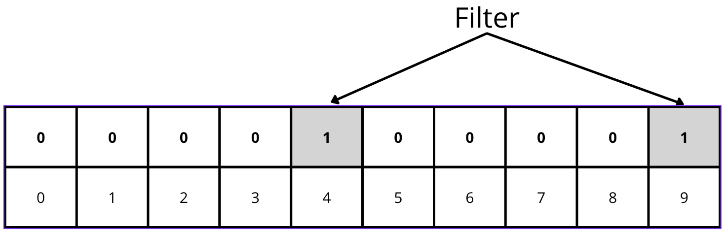
Now we add the word “Filter”, resulting in the hash functions indicating positions 4 and 9:
At this point, we can start making some queries to the data structure.
For example, we query if the element “Bloom” exists. The hash functions will return 0 and 4, the same result as when we performed the insertion. Checking the data structure, we see that both positions have a value of 1. As a result, we can say that the element “Bloom” MIGHT be in the structure.
Now we want to check if the element “Hash” is inside the structure. We apply the hash functions and get positions 3 and 4. We can affirm that the element “Hash” is NOT in the structure because the value of position 3 is 0.
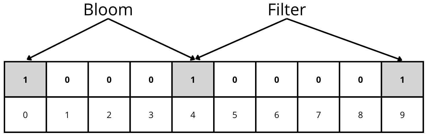
Lastly, we want to check if the element “Function” is stored in the structure. We apply the hash functions and get positions 0 and 9. Checking the data structure, we see that both positions have a value of 1.
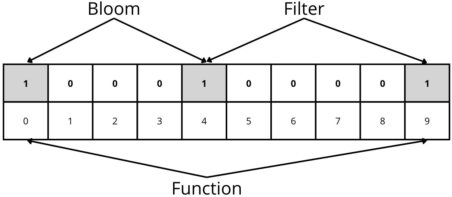
As a result, we can say that the element “Function” MIGHT be in the structure. However, this element is not actually in the structure. This is a false positive because the output values of the hash functions for the element “Function” have collided with the outputs of the hash functions for the elements “Bloom” and “Filter”.
How to use it
Let’s assume we are a social network receiving hundreds of thousands of requests per second. However, the security team has detected that 25% of these requests are malicious and aim to overload our systems and degrade the quality of our service.
The security team has provided us with a list of 1 million IP addresses to develop a firewall that blocks requests from these IPs. They inform us that when these IPs are blocked, the attackers might use others, but they will not exceed 10 million in total.
After testing several solutions with different NoSQL databases, we discard this option because the response times are even slower than before, and moreover, the application is down during the attacks.
We spoke with the product team and reached an agreement: we can block 1% of the non-malicious requests if the remaining 99% of customer requests function correctly.
Given these data and constraints, the Bloom Filter is a great candidate to solve the problem. We need a highly efficient data structure, and we can tolerate an error margin of less than 1%. Moreover, the maximum number of input elements ( IPs) is 10 million.
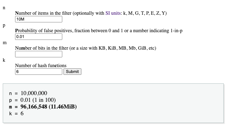
To know exactly the size of the array and the number of hash functions, we can use this calculator. The goal of using the calculator is to find the optimal point of memory usage and hash functions.
In our case, an array of 11.46 MB and 6 hash functions gives us the desired probability of false positives for the required number of entries (IPs):
With these parameters, we can construct the structure and insert all the IPs provided by the security team. Whenever someone makes a request, we will check if the IP is in the structure. Given the probabilistic nature of the solution, there will be false positives, meaning non-malicious users will have their requests blocked. However, there will be no false negatives, meaning a malicious user will not manage to have their request reach our servers.
Counting Bloom Filter
At this point, following the previous example, the security team informs us that they occasionally misclassify IPs. Therefore, they want not only to add malicious IPs but also to remove those that were initially classified as such but ultimately are not.
The classic Bloom Filter solution does not support deletion. Each position in the array is formed by a bit, and thus, each position has a value of 0 or 1. Deleting an element would involve changing the values in the array where the element is stored to 0. However, this cannot be done since we might be removing other elements from the structure.
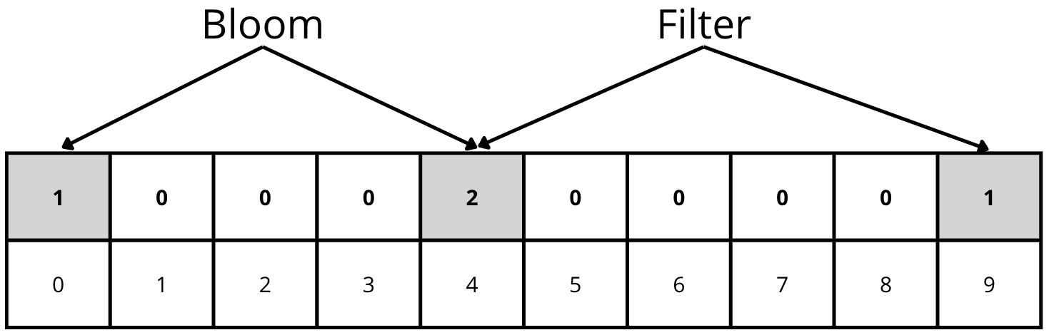
As a solution to this problem, the Counting Bloom Filter was developed. It maintains the classic idea but converts the values in the array into integers that increase with each insertion and decrease with each deletion:
As always, there are no perfect solutions. The classic Bloom Filter is very efficient in terms of memory because each position in the array is a bit. However, the Counting Bloom Filter must store integers, which multiplies the size of the data structure several times.
Computational cost
There are three operations (if we include the Counting Bloom Filter):
- Search
- Insert
- Delete
In all operations, the computational cost is O(h) being h the number of hash functions. Assuming that the hash functions do not vary based on the number of elements within the structure, we can say that the computational cost is constant for all operations, i.e., O(1).
A small (L3) problem
We have seen the characteristics of this probabilistic data structure and on paper, it seems almost perfect. However, data structures must be used in practice and not just presented in papers or conferences.
Normally, data structures are designed assuming infinite computational and memory capabilities. I’m not saying this is wrong in the academic environment, but in practice, we can face reality.
This data structure is designed for use cases that require very high performance. However, we must take into account one thing: the size of this data structure can easily exceed MB levels.
If we consider the access costs to different types of memory (L1, L2, etc.), we will realize that the access cost multiplies by 3 at each layer until reaching memory, at which point the cost multiplies by many times when accessing disk storage.
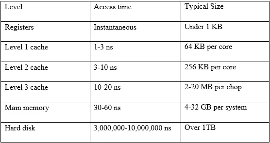
If we have a bit array under 20MB, it is very likely (depending on the CPU) that it can be stored in the processor’s memories, and access to these is extremely fast. However, beyond 20MB, we will hit the wall of memory, which can significantly reduce the performance of this data structure. In certain use cases, accessing memory may be better than any other alternative (for example, accessing disk), but it’s a limitation we must consider.
Use cases
Many significant projects employ or have employed this data structure. Here are some examples:
- Many databases (Bigtable, Cassandra, PostgreSQL, etc.) use Bloom Filters to reduce disk searches for rows or columns that do not exist.
- Medium uses Bloom Filters to avoid recommending articles that users have already read.
- Bitcoin employed Bloom Filters to speed up the synchronization of wallets.